
How to Create a Pivot Table in Excel: At the point when the real pivot table was designed is in question. The Excel group authored the timeframe pivot table, which was respected in Excel in 1993.
Be that as it may, the thought gets not new. Pito Salas and his group at Lotus were taking a shot at the turn work area thought in 1986 and discharged Lotus Improv in 1991. Prior to that point, Javelin gave usefulness much like that of pivot tables.
The focal thought of driving a pivot table is that the data, formulas, and data views are taken care of autonomously. In this post, we explained how to create a pivot table in Excel.
Now that you have a good understanding of the importance of a wellstructured information source, let’s walk through the basic things to create a pivot table in Excel.
To guarantee that the pivot table catches the scope of your information source, of course, click any single cell in your information source. Next, select the Insert tab and discover the Tables gathering.
In the Tables, select PivotTable and afterward pick PivotTable from the dropdown menu. Picture 1.1 shows how to begin a pivot table.

Picture 1.1 Start a pivot table by selecting PivotTable from the Insert tab.
Choosing these options activates the Create PivotTable dialog box, shown in Picture 1.2

Picture 1.2 The Create PivotTable dialog box.
Tips:
You can also press the shortcut to start a pivot table: Press and release Alt, press, and release N, and then press and release V.
As you can see in Picture 1.2, the Create PivotTable dialog box asks you only two fundamental questions:
- Where’s the data that you want to analyze?
- Where do you want to put the pivot table?
Here’s how you handle these two sections of the dialog box:
Choose The Date That You Want To Analyze—In this section, you tell Excel where your data set is. You can specify a data set that is located within your workbook, or you can tell Excel to look for an external data set.
As you can see in Picture 1.2, Excel is smart enough to read your data set and fill in the range for you. However, you always should take note of the range of Excel selects to ensure that you are capturing all your data. Keep in mind that this is the basic thing to create a pivot table in Excel.
Choose Where You Want The PivotTable Report To Be Placed—In this section, you tell Excel where you want your pivot table to be placed. This is set to New Worksheet by default, meaning that your pivot table will be placed in a new worksheet within the current workbook.
You will rarely change this setting because there are relatively few times you’ll need your pivot table to be placed in a specific location.
Note:
The presence of another option in the Create PivotTable dialog box shown in Picture 1.2: Add This Data To The Data Model option. You would select this option if you were trying to consolidate multiple data sources into a single pivot table. In this post, we’ll keep it basic by covering the steps to create a pivot table from using a single source, which means you can ignore this particular option.
After you have answered the two questions in the Create PivotTable dialog box, simply click the OK button. At this point, Excel adds a new worksheet that contains an empty pivot table report. Next to that is the PivotTable Fields list, shown in Picture 1.3. This page helps you build your pivot table.

Picture 1.3 You use the PivotTable Fields list to build a pivot table.
The icons for Columns and Rows in Picture 1.3 are reversed. A summer intern at Microsoft inadvertently reversed the icons several versions ago and no one noticed. After Bill pointed this out to the correct project manager, they pledged to restore the icons to the correct location.
Editor Recommendation:
Formula Examples To Calculate Percentage In Excel
Finding the PivotTable Fields List
The PivotTable Fields list is your main work area in Excel 2020. This is the place where you add fields and make changes to a pivot table report. By default, this page pops up when you place your cursor anywhere inside a pivot table.
However, if you explicitly close this pane, you override the default and essentially tell the pane not to activate when you are in the pivot table.
If clicking on the pivot table does not activate the PivotTable Fields list, you can manually activate it by rightclicking anywhere inside the pivot table and selecting the Show Fields list. You can also click anywhere inside the pivot table and then choose the large Fields List icon on the Analyze tab under PivotTable Tools in the ribbon. [One of the most demanding options for people to create a pivot table in Excel]
Adding fields to a Report
You can add the fields you need to a pivot table by using the four “areas” found in the PivotTable Fields list: Filters, Columns, Rows, and Values. These areas, which correspond to the four areas of the pivot table, are used to populate your pivot table with data:
Filters—Adding a field to the Filter area enables you to filter its unique data items. In previous versions of Excel, this area was known as the Report Filters area.
Columns—Adding a field into the Columns area displays the unique values from that field across the top of the pivot table.
Rows—Adding a field into the Rows area displays the unique values from that field down the left side of the pivot table.
Values—Adding a field into the Values area includes that field in the Values area of your pivot table, allowing you to perform a specified calculation using the values in the field.
Adding Layers to a Pivot Table in Excel
Now you can add another layer of analysis to your report. Say that now you want to measure the number of dollar sales each region earned by product category. Because your pivot table already contains the Region and Sales Amount fields, all you have to do is select the checkbox next to the Product Category field.
As you can see in Picture 1.4, your pivot table automatically added a layer for the Product Category and refreshed the calculations to include subtotals for each region. Because the data is stored efficiently in the pivot cache, this change took less than a second. One of the most important options for people is to create a pivot table in Excel.

Picture 1.4 Without pivot tables, adding layers to analyses requires hours of work and complex formulas.
Rearranging a Pivot table in Excel
Suppose that the view you’ve created doesn’t work for your manager. He wants to see Product Categories across the top of the pivot table report. To make this change, simply drag the Product Category field from the Rows area to the Columns area, as illustrated in Picture 1.5.

Picture 1.5. Rearranging a pivot table is as simple as dragging fields from one area to another.
The report is instantly restructured, as shown in Picture 1.6.

Picture 1.6 Your product categories are now column-oriented.
Creating a Report Filter
You might be asked to produce different reports for particular regions, markets, or products. Instead of building separate pivot table reports for every possible analysis scenario, you can use the Filter field to create a report filter.
For example, you can create a regionfiltered report by simply dragging the Region field to the Filter area and the Product Category field to the Rows area. This way, you can analyze one particular region at a time. Picture 1.7 shows the totals for just the North region.

Picture1.7 With this setup, you not only can see revenues by product clearly but also can click the Region dropdown menu to focus on one region.
UNDERSTANDING THE RECOMMENDED PivotTable AND THE IDEAS FEATURES
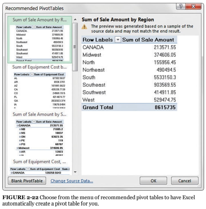
With Excel 2013, Microsoft introduced a feature called Recommended PivotTables. You can find this feature next to the PivotTable icon on the Insert tab (refer to Figure 212). This feature is Microsoft’s way of getting you up and running with pivot tables by simply creating one for you. The idea is simple: Place your cursor in a tabular range of data and then click the Recommended PivotTables icon.
Excel shows you a menu of pivot tables it thinks it can create for you, based on the data in your range (see Figure 2 22). When you find one that looks good to you, click it and then click OK to have Excel create it.
Learn Ideas feature Uses Artificial intelligence to Create a Pivot Table in Excel
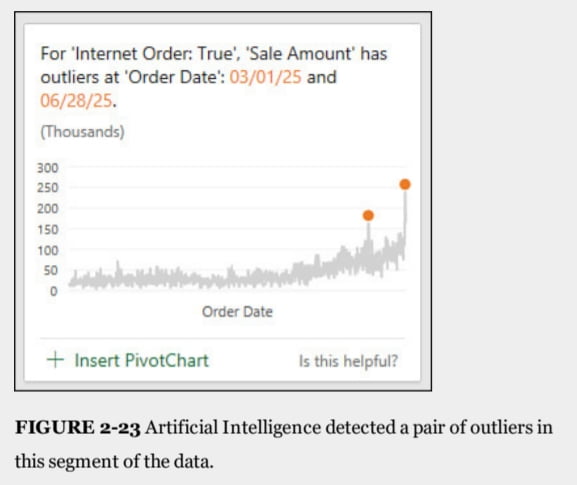
The Recommended PivotTable algorithm is looking for columns with headings of Revenue, Profit, or Sales. If it cannot find any of those, it will use the last numeric column in the data set. The new Ideas feature uses artificial intelligence to analyze up to 250,000 cells of your data.
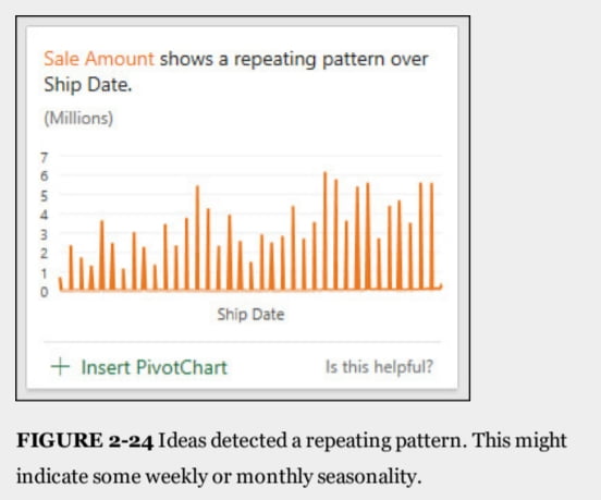
Ideas initially offer descriptive pivot tables like those produced in Recommended PivotTables, but then it offers far more advanced analyses. While the Recommended PivotTables produces 10 choices, the Ideas feature often produces over 30 choices. Figures 223 and 224 show some results available from Ideas.
When the Ideas feature debuted in the summer of 2018, it was called Insights and was found on the Insert tab. By the end of 2018, Office 365 customers would see the feature on the right side of the Home tab, and it was rebranded as Ideas.
Unfortunately, customers who purchased a perpetual license to Excel 2019 will not have the feature in either location. Microsoft’s stance is that if you are not continuing to pay a monthly subscription fee, you cannot make use of the Office intelligent services.
The reviews on the Insert Recommended PivotTables feature are mixed. On one hand, it does provide a quick and easy way to start a pivot table, especially for those of us who are not that experienced.
On the other hand, Excel’s recommendations are rudimentary at best. You will often find that you need to rearrange, add, or manipulate fields in the created pivot table to suit your needs. Although Excel might get it right the first time,
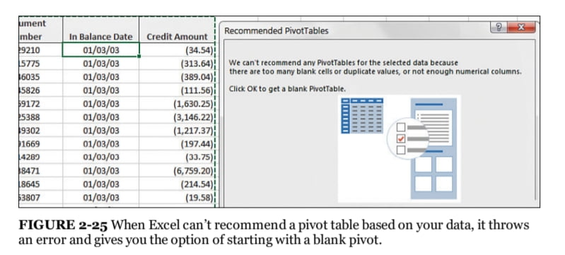
it’s unlikely that you will be able to leave the pivot table as is. There is also a chance that Excel will simply not like the data range you pointed to. For example, the data in Figure 225 is a valid range,
but Excel doesn’t like the repeating dates. So, it pops up a message to indicate that there are too many duplicates to recommend a pivot table; however, it will gladly create a blank one.
All in all, the Recommended PivotTables feature can be a nice shortcut for getting a rudimentary pivot table started, but it’s not a replacement for knowing how to create and manipulate pivot tables on your own.
USING SLICERS
With Excel 2010, Microsoft introduced a feature called slicers. Slicers enable you to filter your pivot table in much the same way as Filter fields filter a pivot table.
The difference is that slicers offer a userfriendly interface that enables you to easily see the current filter state.
Creating a Standard Slicer
To understand the concept behind slicers, place your cursor anywhere inside your pivot table, and then select the Insert tab on the ribbon. Click the Slicer icon (see Figure 2-26).

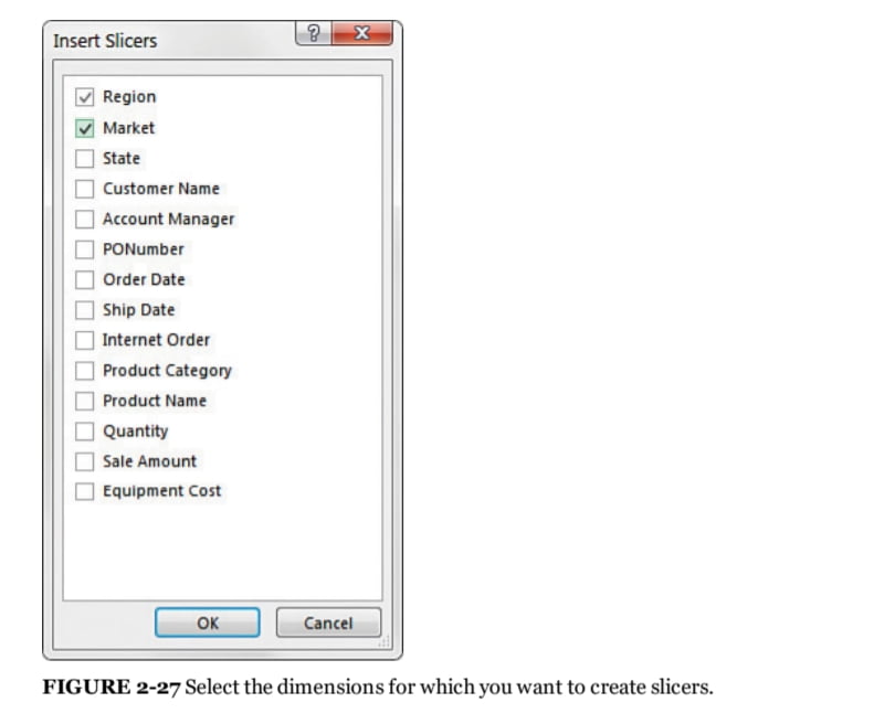
The Insert Slicers dialog box, shown in Figure 2-27, opens. The idea is to select the dimensions you want to filter. In this example, the Region and Market slicers are selected.
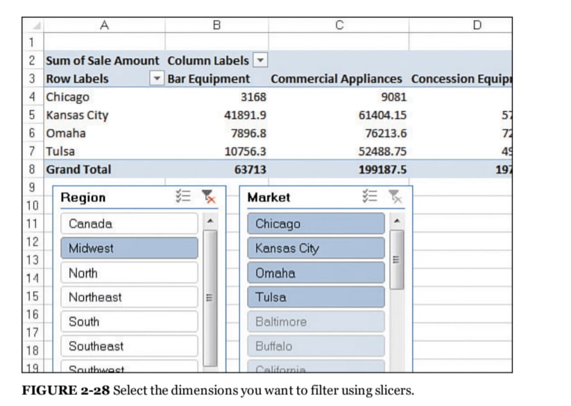
After the slicers are created, you can simply click the filter values to filter your pivot table. As you can see in Figure 228, clicking Midwest in the Region slicer filters your pivot table, and also the Market slicer responds by highlighting the markets that belong to the Midwest region.
TIP:
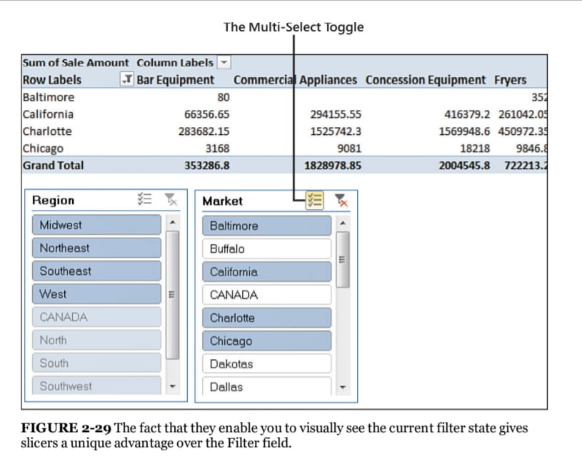
You can select multiple values by holding down the Ctrl key on your keyboard while selecting the needed filters. Alternatively, you can enable the MultiSelect toggle next to the filter icon at the top of the slicer.
In Figure 229, the MultiSelect toggle was enabled and then Baltimore, California, Charlotte, and Chicago were selected. Note that Excel highlights the selected markets in the Market slicer and also highlights their associated regions in the Region slicer.
Another advantage you gain with slicers is that you can tie each slicer to more than one pivot table. In other words, any filter you apply to your slicer can be applied to multiple pivot tables.
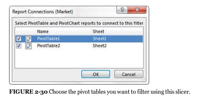
To connect a slicer to more than one pivot table, simply rightclick the slicer and select Report Connections. The Report Connections dialog box, shown in Figure 2-30, opens. Select the checkbox next to any pivot table that you want to filter using the current slicer.
At this point, any filter applied via the slicer is applied to all the connected pivot tables. Again, slicers have a unique advantage over Filter fields in that they can control the filter state of multiple pivot tables. Filter fields can control only the pivot table in which they live.
Tips:
Notice that in Figure 230, the list of pivot tables is a bit ambiguous (PivotTable1, PivotTable2). Excel automatically gives your pivot tables these generic names, which it uses to identify them.
You can imagine how difficult it would be to know which pivot table is when working with more than a handful of pivots. Therefore, you might want to consider giving your pivot tables userfriendly names, so you can recognize them in dialog boxes, such as the one you see in Figure 2-30.
You can easily change the name of a pivot table by placing your cursor anywhere inside the pivot table, select the Analyze tab, and entering a friendly name in the PivotTable Name input box found on the far left.
Creating a Timeline slicer
The Timeline slicer (introduced with Excel 2013) works in the same way as a standard slicer in that it lets you filter a pivot table using a visual selection mechanism instead of the old Filter fields. The difference is that the Timeline slicer is designed to work exclusively with date fields, and it provides an excellent visual method to filter and group the dates in a pivot table.
Tips:
In order to create a Timeline slicer, your pivot table must contain a field where all the data is formatted as dates. This means that your source data table must contain at least one column where all the values are formatted as valid dates. If even only one value in the source data column is blank or not a valid date, Excel does not create a Timeline slicer.
To create a Timeline slicer, place your cursor anywhere inside your pivot table, select the Insert tab on the ribbon, and then click the Timeline icon.
The Insert Timelines dialog box opens, showing you all the available data fields in the chosen pivot table. Here, you select the date fields for which you want to create slicers.
After your Timeline slicer is created, you can filter the data in your pivot table by using this dynamic dataselection mechanism. As you can see in Figure 2-31, clicking the April slicer filters the data in the pivot table to show only April data.
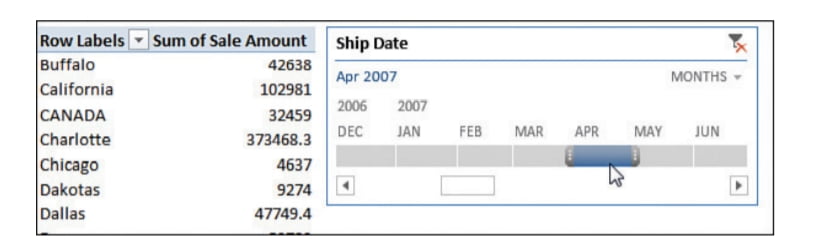
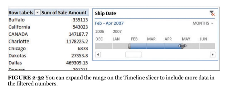
Figure 2-32 demonstrates how you can expand the slicer range with the mouse to include a wider range of dates in your filtered numbers.
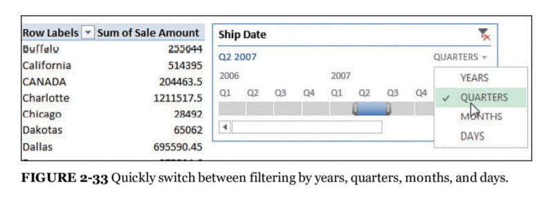
Want to quickly filter your pivot table by quarters? Well, you can easily do it with a Timeline slicer. Click the time period dropdown menu and select Quarters. As you can see in Figure 2-33, you also have the option of selecting Years or Days, if needed.
KEEPING UP WITH CHANGES IN THE DATA SOURCE
Let’s go back to the family portrait analogy. As the years go by, your family will change in appearance and might even grow to include some new members. The family portrait that was taken years ago remains static and no longer represents the family today. So, another portrait needs to be taken.
As time goes by, your data might change and grow with newly added rows and columns. However, the pivot cache that feeds your pivot table report is disconnected from your data source, so it cannot represent any of the changes you make to your date source until you take another snapshot.
The action of updating your pivot cache by taking another snapshot of your data source is called refreshing your data. There are two reasons you might have to refresh your pivot table report:
- Changes have been made to your existing data source.
- Your data source’s range has been expanded with the addition of rows or columns.
The following sections explain how to keep your pivot table synchronized with the changes in your data source.
Dealing with changes made to the existing data source
If a few cells in your pivot table’s source data have changed due to edits or updates, you can refresh your pivot table report with a few clicks. Simply rightclick inside your pivot table report and select Refresh. This selection takes another snapshot of your data set, overwriting your previous pivot cache with the latest data.
NOTE:
You can also refresh the data in a pivot table by selecting Analyze from the PivotTable Tools tab in the ribbon and then choose Refresh.
Tips:
Clicking anywhere inside a pivot table activates the PivotTable Tools tabs just above the main ribbon.
Dealing with an expanded data source range due to the addition of rows or columns
When changes have been made to your data source that affects its range (for example, if you’ve added rows or columns), you have to update the range being captured by the pivot cache.
To do this, click anywhere inside the pivot table and then select Analyze from the PivotTable Tools tab in the ribbon. From here, select Change Data Source. This selection triggers the dialog box shown in Figure 2-35.
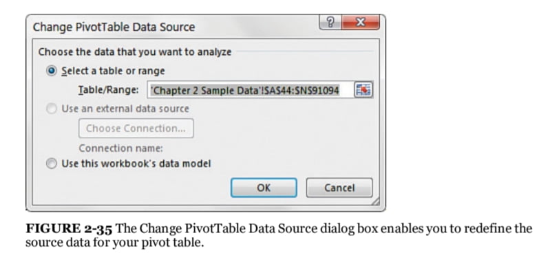
All you have to do here is update the range to include new rows and columns. After you have specified the appropriate range, click the OK button.
Note that if you format your pivot table source data as a table using Home, Format As Table, or Ctrl+T, the Pivot Table Source range will automatically expand as the data grows. You will still have to click Refresh to pick up the new rows.
if the post create a pivot table in excel is helpfull for you,please give us a review